
2.2.1 General modelling approach
This section describes the general approach of our models and the methodology used to estimate Scope 1, 2, and 3 carbon operational emissions[1], the carbon footprint, and the carbon intensity and efficiency of infrastructure assets across 60+ asset subclasses.
Generally, we can apply our modelling approach to all types of infrastructures. Although infrastructure assets can be significantly different in their function, characteristics, employed technologies, and size, they share enough common features (e.g., relying on fuel to offer a product or service, serving the needs of the general population, generating waste during their activities etc.) to build a framework that can be applied to all types of infrastructure assets.
However, we adjusted our general framework depending on the type of sector and its respective activities. Accordingly, our methodology relies heavily on the TICCS taxonomy to estimate emissions and calculate carbon intensity for different asset sectors. With its classification of asset subclasses, industrial classes, and superclasses, TICCS provides a precise description of each sector’s activities and hence, serves as a basis for our modelling approach.
Furthermore, we assume that some of the assets’ physical characteristics remain unchanged (e.g., the length of a road, the area of a building, or the capacity of a power plant are unlikely to change over a short period). Based on this understanding, we group asset sectors based on similar activities on the superclass (e.g., IC20 – waste and water treatment), industrial class (e.g., IC4010 – pipelines), and subclass level (e.g., IC601010 – airports). For each of these groups, we built a model to predict emissions on an annual basis.
Overall, we differentiate between two types of models: Based on data availability, we built regression-based models (RBMs) or activity-based models (ABMs). RBMs combine reported emissions with one or more asset-level characteristics that correlate well with emission levels to build statistical models. ABMs use tested emission factors (EFs) and capacity (CFs) or consumption (CoFs) factors to convert an asset’s activity and usage into calculated emissions and hence, do not rely on reported emissions (see Figure). In general, ABMs employ characteristics that relate to the operational reality of assets. In comparison, RBMs can include operational characteristics as well as physical features in the regression of reported emissions.
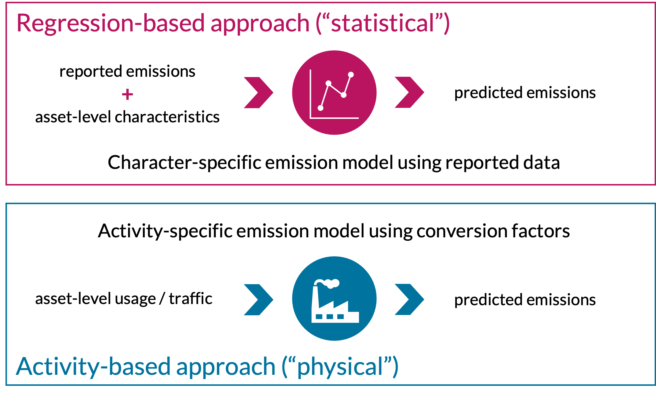
Regression-based and activity-based models to estimate emissions (own illustration)
We apply these models to a representative sample of assets of the Unlisted Infrastructure Universe for which infraMetrics tracks financial information. We combine predicted and reported emissions while prioritising reported emissions, assuming they were calculated based on more data and better knowledge of an asset’s operation. Aggregations of scopes (e.g., sums of Scope 1 and 2 or Scope 1, 2, and 3 emissions) allow us to constitute assets’ carbon footprints. Accordingly, infrastructure investors can use our predictions to construct sector-level benchmarks and assess the emissions of their assets in comparison to TICCS’ superclass, industrial class, and subclass level.
Finally, we used the Scope 1, 2, and 3 emissions and infraMetrics financial information to produce several climate impact and risk measures. Those metrics include absolute and financed carbon emissions, carbon intensity based on a company’s revenue and total assets, and measures of current and future transition risk.
Model valuation
We evaluate the quality (or robustness) of our models based on a panel of methods and tests that depend on the nature of the input data, the volume of reported emissions, and the model type.
For ABMs, we exclude reported emissions because of the lack of data volume and quality and the better performance of our models. Hence, the models rely on the quality of the EFs, CFs, and CoFs used. Since these factors can be established from the literature (top-down approach) or directly from the data (bottom-up approach), they can partly be tested in order to evaluate the quality of predictions. Also, predicted emissions can be compared to reported data and used for out-of-sample residual analyses to validate models.
For RBMs, the methodology involves reported data to calibrate model parameters. Hence, estimated emissions can be compared to the data used during model calibration. This comparison can be used for in-sample residual analyses and tests of normality. In addition, other methods can be applied to validate the model quality: For example, the emissions predictions for assets with reported emissions allow us to conduct out-of-sample residual analyses. When the volume of reported emissions is low, we can compare estimated values with reported emissions found in sustainability reports.
It needs to be noted that some of the reported emissions are aggregated emissions on the company, not on the asset level. Such cases have been selected for some models to verify the accuracy of asset-level predictions when summed over and compared to multi-asset companies’ reported emissions.
Overall, our model design is aligned with the PCAF’s Global GHG Accounting and Reporting Standard. Accordingly, our models receive a PCAF score.
[1] The “carbon operational emissions” refer to the lifecycle of an infrastructure asset – from its construction to its operational process and its decommissioning. For our modelling approach, we include only those carbon emissions produced during an asset’s operational phase. For simplicity, we refer to the carbon operational emissions as ‘emissions’ or ‘carbon emissions.’