Profitability filters

Performing an exercise similar to size filters is not feasible for profitability as private equity focuses on acquiring companies that are ripe for transformation, thus not shying away from unprofitable companies. So outliers present opportunity rather than discouraging PE. Thus, we focus on mapping the profitability profiles of the two samples, i.e., the transactions and the privateMetrics® database.

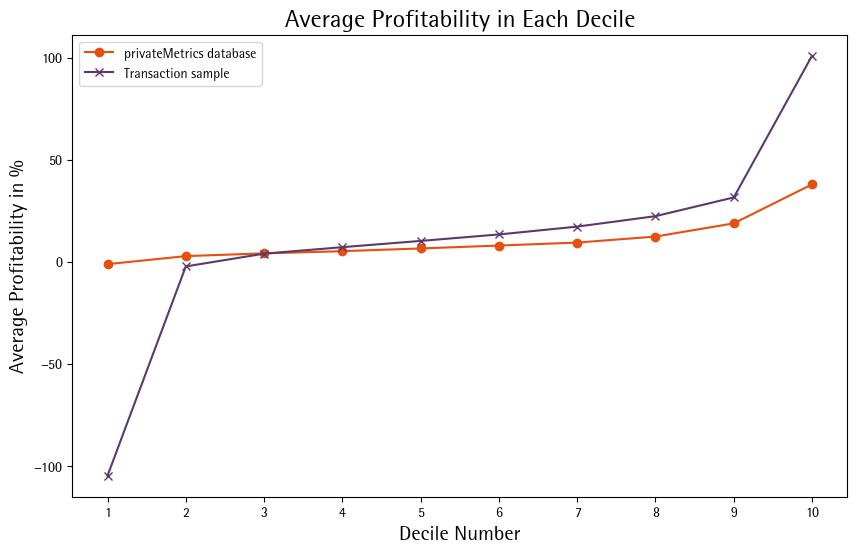
To get a sense of the profitability profiles in the two samples, we segment the ratio of EBITDA to Sales into deciles in each sample and compute the average within each decile. The results are produced in the below plot. Ignoring the outliers in transactions, what stands out is the steepness in how profitability increases as we move across deciles in the Transaction sample, whereas it is quite flat in the privateMetrics® database.

In terms of outliers, the privateMetrics® database is fairly well-behaved, even in contrast to the transactions sample. However, there are a large number of low profitable companies that are dragging the slope of the curve above, and these warrant being excluded.

In other words, there are a lot of “boring private companies”, which Private Equity managers are never going to consider. Once these are excluded, the slope of the privateMetrics® database will be similar to that of the transactions sample.

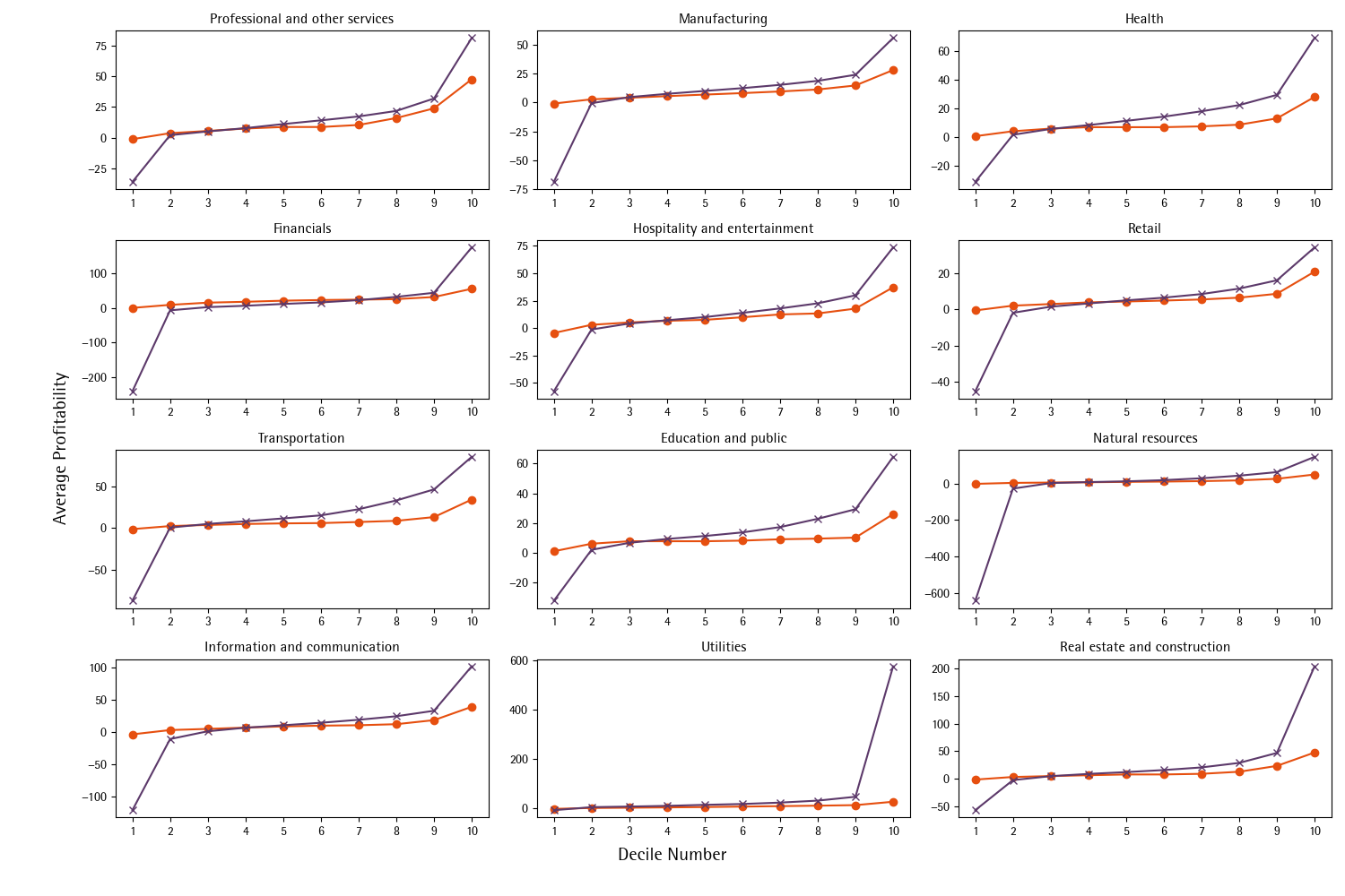
Furthermore, given that profitability varies systematically with sectors, we propose to identify boring companies in each sector so that the average profitability across deciles in that sector in the privateMetrics® database resembles that in transactions in the sector. This is made clear in the plot below, where repeating the exercise by PECCS™ industrial activity produces differences in how much the profitability profiles deviate by sector.

Now to achieve a profit profile that resembles that of the transaction sample, two key steps are required:

1. Filter: Identifying an appropriate filter that can move the profit profile towards the transaction sample for each sector.

2. Metric: Computing a metric that can summarise the extent of alignment of the two curves, ignoring the outliers.

For step 1, we experiment with filters beginning from various starting points and ranging for different bandwidths. Given the evidence in the full sample, we play around with filters ranging from -20% profitability to +15% profitability and alter bandwidths in increments of 1 % till a maximum bandwidth of 15%. This gives rise to several combinations of filters, which, when applied to the universe, allow us to compare the profit profile with that of the profit profile of transactions.

For step 2, we simply sum up the squared differences between the two curves, ignoring the first and the tenth decile. We call our metric SSD or the sum of squared differences in profitability between the two samples, and we proceed to minimize the SSD in each sector. SSD is computed as below:

where μ is the average in each sector i of the profitability Profit measured as the EBITDA to sales ratio, within the decile (d) defined by the same profitability ratio in the two samples, namely the Deals (or transaction) sample and the Universe (or privateMetrics® database), respectively. We exclude the first and the tenth decile in the sum to ignore the effect of outliers in the Deals sample. For the Universe sample, the mean takes into account the filter specifications by excluding companies whose Profit falls within the range of ft_st or filter starting value and ft_st+bw or filter starting value plus the bandwidth of the filter.

Finding the optimal filters then becomes a minimization problem, where we identify both a global minimum, which is the minimum SSD value across all combinations of filters, and several local minima, which are the minimum SSD values for each bandwidth of the filter. Local minima are useful substitutes as in some sectors, the global SSD minimum might leave out too few private companies in the database, in which case we can choose one of the local minima of SSD.

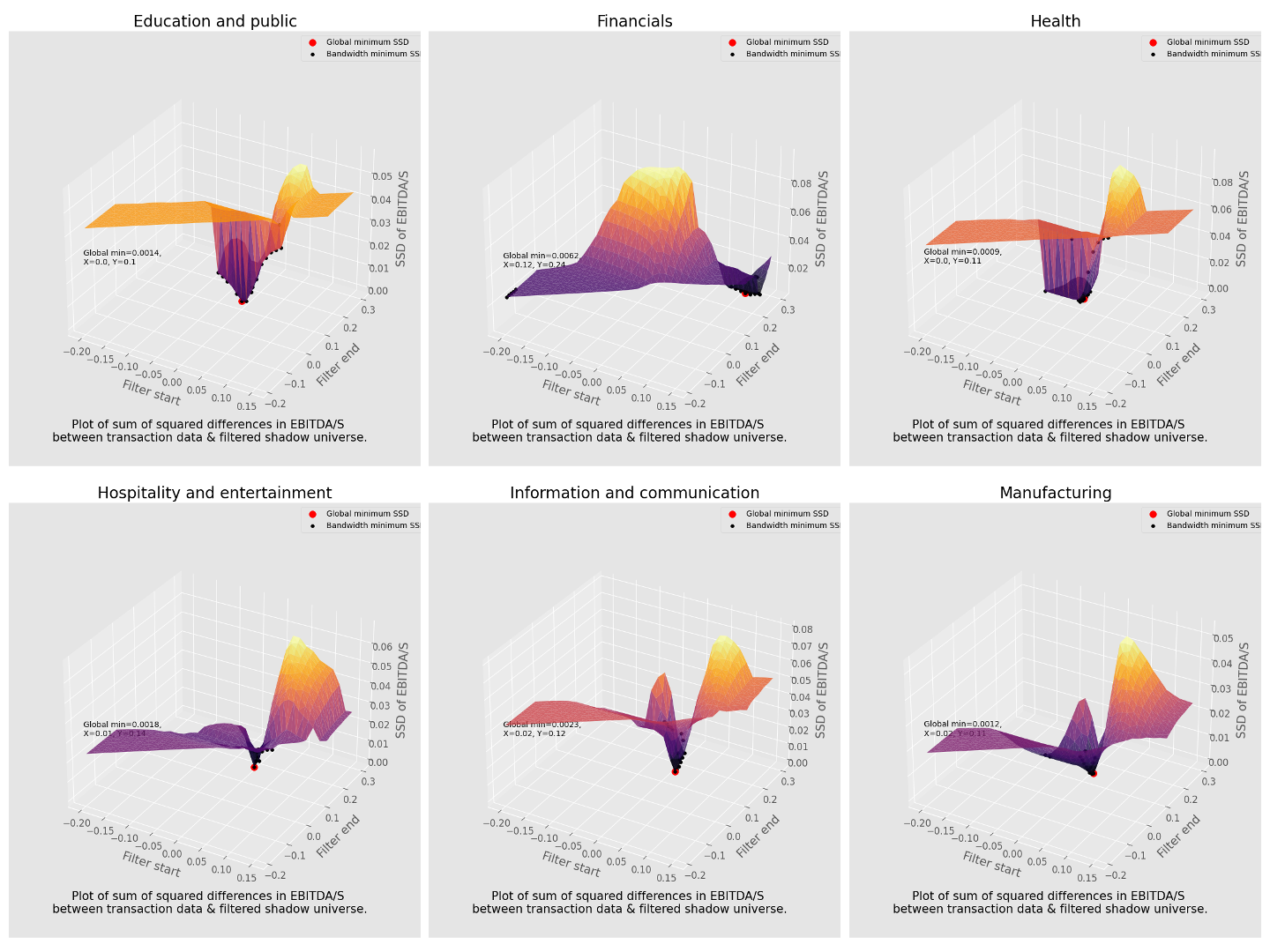
The results of these optimizations at the sector level are reproduced in the images below. The z-axis represents the SSD value, while the x- and y-axes correspond to the filter starting and ending values. The plotted plane represents the values of SSD that correspond to each filter, with the colour of the plane ranging from dark to light with the value of SSD. The red dot indicates a global minimum SSD for each sector and the black dots represent the local minima at each filter bandwidth for each sector.

Thus, this approach leads to the identification of several filter combinations at the sector level for EBITDA/S, which can lead to a profit profile of the privateMetrics® database that almost resembles that of the transactions data in private markets.

In conclusion, we choose a filter that balances coverage requirements with having a low SSD, leading to the identification of the PEU or Private Equity-backed Universe.