
1.2.1 Valuation Approaches
A. Market-based Approaches
Market-based approaches to valuation rely on using market related inputs such as the valuation of similar publicly listed peers or recent transactions to arrive at an estimated valuation. Also known as “Comps” analysis, it is very popular to apply a listed sector or listed/unlisted peers’ price multiples (e.g., P/S, P/Ebitda, or EV/Ebitda) to a focal private company to arrive at its valuation.
Counter-intuitively, comps analysis is also a form of model-based approach. For example, we can see it as a simplified form of the dividend discount model (DDM). The traditional single-period model can be stated as in the below equation where P is the valuation, D1 is the dividend next period, and r and g are the required return and sustainable growth rate, respectively.
' aria-hidden='true'%3e %3cg transform='translate(167%2c0)'%3e %3cg transform='translate(-11%2c0)'%3e %3cg transform='translate(10605%2c4738)'%3e %3cuse xlink:href='%23E1-MJMATHI-50' x='0' y='0'%3e%3c/use%3e %3cuse xlink:href='%23E1-MJMAIN-3D' x='1029' y='0'%3e%3c/use%3e %3cg transform='translate(1807%2c0)'%3e %3cg transform='translate(397%2c0)'%3e %3crect stroke='none' width='2274' height='60' x='0' y='220'%3e%3c/rect%3e %3cg transform='translate(496%2c819)'%3e %3cg%3e%3c/g%3e %3cuse xlink:href='%23E1-MJMATHI-44' x='0' y='0'%3e%3c/use%3e %3cuse transform='scale(0.707)' xlink:href='%23E1-MJMAIN-31' x='1171' y='-213'%3e%3c/use%3e %3c/g%3e %3cg transform='translate(60%2c-880)'%3e %3cg%3e%3c/g%3e %3cuse xlink:href='%23E1-MJMATHI-72' x='0' y='0'%3e%3c/use%3e %3cuse xlink:href='%23E1-MJMAIN-2212' x='673' y='0'%3e%3c/use%3e %3cuse xlink:href='%23E1-MJMATHI-67' x='1674' y='0'%3e%3c/use%3e %3c/g%3e %3c/g%3e %3c/g%3e %3c/g%3e %3cg transform='translate(8006%2c1579)'%3e %3cuse xlink:href='%23E1-MJMATHI-50' x='0' y='0'%3e%3c/use%3e %3cuse xlink:href='%23E1-MJMAIN-3D' x='1029' y='0'%3e%3c/use%3e %3cg transform='translate(1807%2c0)'%3e %3cg transform='translate(397%2c0)'%3e %3crect stroke='none' width='4874' height='60' x='0' y='220'%3e%3c/rect%3e %3cg transform='translate(60%2c819)'%3e %3cg%3e%3c/g%3e %3cuse xlink:href='%23E1-MJMATHI-45' x='0' y='0'%3e%3c/use%3e %3cuse transform='scale(0.707)' xlink:href='%23E1-MJMAIN-31' x='1044' y='-213'%3e%3c/use%3e %3cuse xlink:href='%23E1-MJMAIN-D7' x='1414' y='0'%3e%3c/use%3e %3cuse xlink:href='%23E1-MJMATHI-44' x='2415' y='0'%3e%3c/use%3e %3cuse xlink:href='%23E1-MJMATHI-50' x='3243' y='0'%3e%3c/use%3e %3cuse xlink:href='%23E1-MJMATHI-52' x='3995' y='0'%3e%3c/use%3e %3c/g%3e %3cg transform='translate(1359%2c-880)'%3e %3cg%3e%3c/g%3e %3cuse xlink:href='%23E1-MJMATHI-72' x='0' y='0'%3e%3c/use%3e %3cuse xlink:href='%23E1-MJMAIN-2212' x='673' y='0'%3e%3c/use%3e %3cuse xlink:href='%23E1-MJMATHI-67' x='1674' y='0'%3e%3c/use%3e %3c/g%3e %3c/g%3e %3c/g%3e %3c/g%3e %3cg transform='translate(0%2c-1580)'%3e %3cuse xlink:href='%23E1-MJMATHI-50' x='0' y='0'%3e%3c/use%3e %3cuse xlink:href='%23E1-MJMAIN-3D' x='1029' y='0'%3e%3c/use%3e %3cg transform='translate(1807%2c0)'%3e %3cg transform='translate(397%2c0)'%3e %3crect stroke='none' width='12880' height='60' x='0' y='220'%3e%3c/rect%3e %3cg transform='translate(60%2c819)'%3e %3cg%3e%3c/g%3e %3cuse xlink:href='%23E1-MJMATHI-53' x='0' y='0'%3e%3c/use%3e %3cuse transform='scale(0.707)' xlink:href='%23E1-MJMAIN-31' x='867' y='-213'%3e%3c/use%3e %3cuse xlink:href='%23E1-MJMAIN-D7' x='1289' y='0'%3e%3c/use%3e %3cuse xlink:href='%23E1-MJMATHI-50' x='2290' y='0'%3e%3c/use%3e %3cuse xlink:href='%23E1-MJMATHI-72' x='3041' y='0'%3e%3c/use%3e %3cuse xlink:href='%23E1-MJMATHI-6F' x='3493' y='0'%3e%3c/use%3e %3cuse xlink:href='%23E1-MJMATHI-66' x='3978' y='0'%3e%3c/use%3e %3cuse xlink:href='%23E1-MJMATHI-69' x='4529' y='0'%3e%3c/use%3e %3cuse xlink:href='%23E1-MJMATHI-74' x='4874' y='0'%3e%3c/use%3e %3cuse xlink:href='%23E1-MJMATHI-6D' x='5458' y='0'%3e%3c/use%3e %3cuse xlink:href='%23E1-MJMATHI-61' x='6337' y='0'%3e%3c/use%3e %3cuse xlink:href='%23E1-MJMATHI-72' x='6866' y='0'%3e%3c/use%3e %3cuse xlink:href='%23E1-MJMATHI-67' x='7318' y='0'%3e%3c/use%3e %3cuse xlink:href='%23E1-MJMATHI-69' x='7798' y='0'%3e%3c/use%3e %3cg transform='translate(8144%2c0)'%3e %3cuse xlink:href='%23E1-MJMATHI-6E' x='0' y='0'%3e%3c/use%3e %3cuse transform='scale(0.707)' xlink:href='%23E1-MJMAIN-31' x='849' y='-213'%3e%3c/use%3e %3c/g%3e %3cuse xlink:href='%23E1-MJMAIN-D7' x='9420' y='0'%3e%3c/use%3e %3cuse xlink:href='%23E1-MJMATHI-44' x='10421' y='0'%3e%3c/use%3e %3cuse xlink:href='%23E1-MJMATHI-50' x='11249' y='0'%3e%3c/use%3e %3cuse xlink:href='%23E1-MJMATHI-52' x='12001' y='0'%3e%3c/use%3e %3c/g%3e %3cg transform='translate(5362%2c-880)'%3e %3cg%3e%3c/g%3e %3cuse xlink:href='%23E1-MJMATHI-72' x='0' y='0'%3e%3c/use%3e %3cuse xlink:href='%23E1-MJMAIN-2212' x='673' y='0'%3e%3c/use%3e %3cuse xlink:href='%23E1-MJMATHI-67' x='1674' y='0'%3e%3c/use%3e %3c/g%3e %3c/g%3e %3c/g%3e %3c/g%3e %3cg transform='translate(1930%2c-4739)'%3e %3cg transform='translate(120%2c0)'%3e %3crect stroke='none' width='871' height='60' x='0' y='220'%3e%3c/rect%3e %3cg transform='translate(60%2c819)'%3e %3cg%3e%3c/g%3e %3cuse xlink:href='%23E1-MJMATHI-50' x='0' y='0'%3e%3c/use%3e %3c/g%3e %3cg transform='translate(113%2c-880)'%3e %3cg%3e%3c/g%3e %3cuse xlink:href='%23E1-MJMATHI-53' x='0' y='0'%3e%3c/use%3e %3c/g%3e %3c/g%3e %3cuse xlink:href='%23E1-MJMAIN-3D' x='1389' y='0'%3e%3c/use%3e %3cg transform='translate(2167%2c0)'%3e %3cg transform='translate(397%2c0)'%3e %3crect stroke='none' width='10590' height='60' x='0' y='220'%3e%3c/rect%3e %3cg transform='translate(60%2c819)'%3e %3cg%3e%3c/g%3e %3cuse xlink:href='%23E1-MJMATHI-50' x='0' y='0'%3e%3c/use%3e %3cuse xlink:href='%23E1-MJMATHI-72' x='751' y='0'%3e%3c/use%3e %3cuse xlink:href='%23E1-MJMATHI-6F' x='1203' y='0'%3e%3c/use%3e %3cuse xlink:href='%23E1-MJMATHI-66' x='1688' y='0'%3e%3c/use%3e %3cuse xlink:href='%23E1-MJMATHI-69' x='2239' y='0'%3e%3c/use%3e %3cuse xlink:href='%23E1-MJMATHI-74' x='2584' y='0'%3e%3c/use%3e %3cuse xlink:href='%23E1-MJMATHI-6D' x='3168' y='0'%3e%3c/use%3e %3cuse xlink:href='%23E1-MJMATHI-61' x='4046' y='0'%3e%3c/use%3e %3cuse xlink:href='%23E1-MJMATHI-72' x='4576' y='0'%3e%3c/use%3e %3cuse xlink:href='%23E1-MJMATHI-67' x='5027' y='0'%3e%3c/use%3e %3cuse xlink:href='%23E1-MJMATHI-69' x='5508' y='0'%3e%3c/use%3e %3cg transform='translate(5853%2c0)'%3e %3cuse xlink:href='%23E1-MJMATHI-6E' x='0' y='0'%3e%3c/use%3e %3cuse transform='scale(0.707)' xlink:href='%23E1-MJMAIN-31' x='849' y='-213'%3e%3c/use%3e %3c/g%3e %3cuse xlink:href='%23E1-MJMAIN-D7' x='7130' y='0'%3e%3c/use%3e %3cuse xlink:href='%23E1-MJMATHI-44' x='8131' y='0'%3e%3c/use%3e %3cuse xlink:href='%23E1-MJMATHI-50' x='8959' y='0'%3e%3c/use%3e %3cuse xlink:href='%23E1-MJMATHI-52' x='9711' y='0'%3e%3c/use%3e %3c/g%3e %3cg transform='translate(4217%2c-880)'%3e %3cg%3e%3c/g%3e %3cuse xlink:href='%23E1-MJMATHI-72' x='0' y='0'%3e%3c/use%3e %3cuse xlink:href='%23E1-MJMAIN-2212' x='673' y='0'%3e%3c/use%3e %3cuse xlink:href='%23E1-MJMATHI-67' x='1674' y='0'%3e%3c/use%3e %3c/g%3e %3c/g%3e %3c/g%3e %3c/g%3e %3c/g%3e %3c/g%3e %3c/g%3e %3c/svg%3e)
|
The dividend can further be expressed as a product of an earnings measure E1 (e.g., net income or free cash flow) and the payout ratio (DPR). E1 further can be expressed as a product of the sales in the next year S1 and the profit margin. If we ignore the difference between the trailing and leading period revenue, we get an expression for the P/S ratio in terms of DDM inputs.
When a peer’s multiple is projected on a company, it is comparable to assuming that the two companies have similar profit margins, retention rates, required returns, and growth rates in the DDM framework. Thus, it is possible to imagine the comps analysis to be an implicit dividend discount model.
In the end, comps analysis is a very powerful method to perform valuation, as it relies on the closest observable proxy to arrive at the valuation. However, the way it is applied in practice, especially in terms of the quality and quantity of inputs, is problematic, as described below:
Known differences between the company and its peers: The implicit assumption of comps is that the focal private company faces identical risk factors and identical sensitivities to those risk factors as the peer(s). However, there could be known systematic differences between the companies which are not accounted for when using its multiple. Subjective adjustments for known differences, discussed separately, create further problems.
Low quantity of inputs used: Only price multiples are used when more information about the focal company and its peers is available.
Low quality of inputs: The use of both handpicked peers and a custom list of transactions allows flexibility in choice to present a valuation as one pleases. Furthermore, when using transaction data, due to the unavailability of a large sample, stale transactions may be included further reducing the utility of this approach.
Adhoc adjustments: Sometimes, to account for differences between a company and its peer, say on account of illiquidity, size, leverage, etc., practitioners may introduce adhoc adjustments to the price multiples. These adjustments are informal and subjective and not driven by theory or data, thus making the valuation uninformative and possibly misleading decision-making for investors.
B. Income-based Approaches
Income-based approaches to valuation rely on using past or expected cash flows from the company adjusted for the level of uncertainty in realising these cash flows. A popular income-based approach to valuations is using the DCF method. DCF uses a simple model of discounting future cash flows and needs expected cash flows, discount rates, and terminal values as inputs. Since private companies can be regarded as going concerns, terminal value computations can be further simplified based on Gordon’s growth model (or DDM) assuming steady growth at terminal horizons. How tenuous are the perpetual growth assumptions is a question worth pondering over.
Thus, applications additionally require a horizon and terminal growth rates. DCF approach is a strong tool to estimate valuation, grounded in theory, and simplistic to apply. However, in practice, some problems emerge in applications of DCF for the valuation of private companies including:
Highly specific inputs: Most of the inputs to DCF are company-specific. Like for example, DCF analysis requires modelling of future revenue, expenses, depreciation, and investment to arrive at free cash flows. Such intensive and uncertain input requirements provide a high level of flexibility for the one using DCF. Often in practice, it is possible to work your way backward from a valuation to choosing a discount rate and cash flow streams that seem reasonable, defeating the purpose of coming up with an objective valuation.
Incorrect discount rates: Often in DCF analysis of private companies, fund managers use each fund’s target IRR as discount rates. This is highly inappropriate as the discount rate is supposed to account for each company’s risk and cannot be based on a one-size-fits-all approach.
C. Frequency of Valuations
Apart from the valuation approaches, it is also important at what frequency the valuation is performed. Currently, valuation is performed at a low frequency that is uninformative for asset allocation strategies. Low-frequency valuations might be a symptom of a combination of factors including choosing the valuation method and the associated input and skill requirements to perform it. For example, third-party fairness opinions on valuations can cost GPs up to $300,000 per opinion (Bloomberg Law, 2023), indicating that this could be a fairly expensive exercise if done frequently involving external parties. Moreover, lack of regulation and LP tolerance leads to most funds estimating valuations at a quarterly or semi-annual frequency.
However, investors not knowing the valuation frequently does not decrease the inherent risk in an asset class, protect the investor, or help their decision-making. On the contrary, low-frequency valuations paint an unrealistic picture of the risk of investing in private markets, showing them as less volatile, safer, and stable investments. Thus, even if estimation problems are ignored for the moment, the frequency of valuations by themselves can produce distortions.
To illustrate this point further, in the below figure, the returns and index levels of the S&P 500 are plotted at different frequencies. Specifically, they are plotted at monthly, quarterly, annual, once in two years, and once in four-year frequencies. In other words, if investors willingly stay uninformed of the S&P 500 performance at higher frequencies and only observe at a preferred lower frequency, then the figure presents what they will observe. Additionally, to facilitate asset class choices, both the annualised Sharpe ratios and maximum drawdowns are included for each frequency.
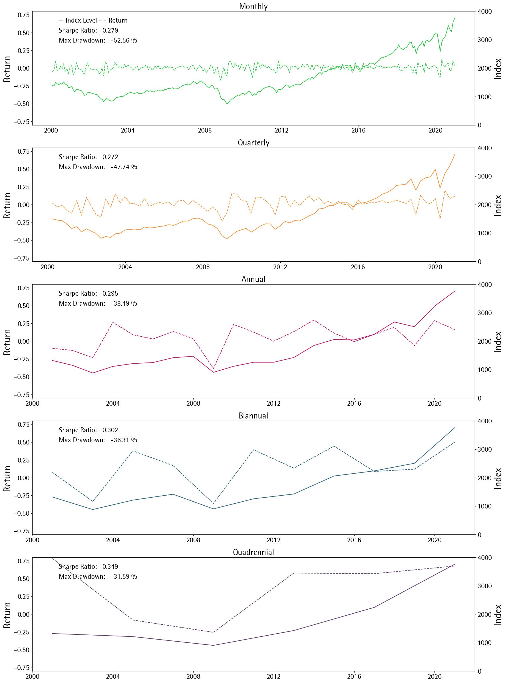
S&P 500 Performance Observed at Different Frequencies
If an asset allocator is asked to choose an asset class just using this data, there will likely be a tendency to choose the asset class represented by lower frequencies as it seems that they are less risky, have fewer periods of negative returns, and perform really well in some periods. These takeaways are also captured in their annualized Sharpe ratios and maximum drawdown measures, which are monotonically increasing and decreasing, respectively, as frequencies go down.
This is the typical issue with private markets when valuations are neither available frequently nor reliable, which understates the risk and burnishes performance. And this exercise illustrates clearly some investors’ perception of private markets.
Bloomberg Law (2023). Private Equity's Fourth Exit Crimped by SEC Plan, Lawyers Say. Bloomberg Law. Accessed July 17, 2024. https://news.bloomberglaw.com/business-and-practice/private-equitys-fourth-exit-crimped-by-sec-plan-lawyers-say.